
Help and methods · 11
Comparing, exporting, sharing and saving
The interface offers several ways to keep your work: a comparison of two dates or products on the map, the data and figure of any card in the formats of your choice, a publication report of several results, an image of the map, a link that reproduces the view, and a saved analysis definition that reconstructs the whole investigation in a later session.
Keeping Hovmöller sections
Each of the four Hovmöller cards offers its own figure and data downloads. Arrange, Dock, Minimise and Restore retain completed results during the visit. The full four-section collection is not yet stored in a shared link or saved-analysis definition. Export the individual results before closing the page. Chart zoom is temporary and is not restored by a link or browser refresh.
Compare maps
Compare maps, under Explore in the left column, opens compact Left (A) and Right (B) controls. Choose a layer and date independently for each side, then Apply. Trend maps have separate periods of at least ten complete years; seven-day change uses its labelled published interval. The right-side presets compare A with its 1991–2020 seasonal SST reference or with the same calendar day of the previous year. Each side has its own legend. The divider drags with the pointer; arrow keys move it in steps of five per cent, and Home and End move it to the edges. Unavailable dates produce an explicit error, not a substitute field.

- 1Left and right layer, date and presets.
- 2The divider.
Download the figure you are viewing
Use Download figure beside a chart to save that individual figure with its current layers, axes and legend. Under Setup → Figure downloads, choose PNG at 1,200, 2,400 (the default) or 4,800 pixels wide, or SVG for vector charts. Height, text, symbols and line widths scale together, preserving the proportions on the screen. Hovmöller and warming stripes use PNG when SVG is your preference; a Hovmöller download includes its colour legend and redraws its axes at the chosen resolution. This improves image detail, not the resolution of the scientific observations.
Files are named for the analysis, location or section endpoints, and the plotted dates, for example saoce_seasonal-cycle_28.320s_9.560e_1991-01-01_to_2026-10-04.png. Each pinned figure and event-evolution panel has its own action. Preferences persist in this browser across visits and workspace Reset; use Restore figure download defaults to restore PNG at 2,400 pixels. A 2,400-pixel image can be placed at 20.3 cm wide at 300 pixels per inch. Right-click saving continues to use the browser’s image representation and naming; use the figure button for these export settings. Reports and map images retain their separate layouts.
Preparing a journal figure
Under Setup → Figure downloads, choose Journal figure and a single-column (85 mm) or double-column (180 mm) starting size. Adjust the final width, text size and 300/600 dpi to the journal’s requirements. Each chart is laid out again at the final physical size on white, in Arial with black text; increasing dpi changes the pixel density, not the lettering size. Statistical line weights are 0.6–1 pt, with lighter grid lines. SVG retains editable lines and text and declares its width and height in millimetres; PNG includes its print-resolution metadata. Keep the file at that size when inserting it into the manuscript. Subsequent scaling changes its lettering too.
Height follows the figure’s proportions up to 170 mm. Download panels individually if a combined card export exceeds that height. Captions, method descriptions and statistical qualifications belong in the manuscript or accompanying report, not inside a cramped plot. Inspect the result at its intended printed size, especially for dense legends, heatmaps or long axis labels. A standard font is referenced in SVG; ensure it is available when editing or converting the file. PNG preserves the rendered typeface.
Requirements vary: Nature’s figure guide specifies 89/183 mm widths and 5–7 pt lettering, whereas PLOS Biology specifies 8–12 pt lettering, 300–600 dpi and TIFF/EPS delivery. These presets support preparation; they do not certify compliance. If the journal requires TIFF or EPS, convert the supplied PNG or SVG without resizing and check the converted file. Full reports and their multi-panel composer retain their own page layouts; the individual chart buttons provide final-size journal exports.
Graph options on every card
Every result card, including the line profile, Hovmöller and distance cards, carries a Graph options menu (the three dots in its header). Export plotted data saves exactly the values on the figure, with their units and the selection, interval, method and lineage: as CSV (a ZIP of CSV files with a README when the figure needs several tables, for example events and the daily series), as netCDF-4 written by the calculation service from those same rows with CF-style attributes (a time-by-distance field for a Hovmöller section), or as JSON. Export figure saves the figure as drawn on the card, as an SVG with editable vector lines and text or as a PNG at your saved output width; the Hovmöller diagram is a raster and exports as PNG. Copy figure places the same PNG on the clipboard, ready to paste into a document or message. Nothing is recomputed or filled for an export; missing days stay missing. Remove card closes the card.
On a marine heatwave or cold-spell card, the events table holds one row per event with its start, peak and end dates, duration, category and category proportions, intensities (relative to the climatology, to the threshold and absolute) and onset and decline rates. The daily table holds the area-mean SST, the event threshold (90th percentile for heatwaves, 10th for cold-spells) and the departure from that threshold for every day of the interval. Download daily SST, threshold and departure (CSV), under the card’s Details, tables and downloads, saves the same daily columns as one file; for the SST alone over any period, switch the card to Daily SST series.

| Export | Contents |
|---|---|
| CSV | One table per dimension: the daily series, annual values, events, bins, fitted curves. Column headers carry the units. |
| netCDF-4 | The same tables as variables on their own dimensions, with the selection, interval, method, lineage and baseline as global attributes. |
| JSON | The tables with their column definitions and attributes. |
| SVG, PNG | The figure as drawn, with its axis titles and units. |
Publication report (PDF)
Under Chart comparison & downloads, Publication report (PDF)… lists every open card with its current method and lets you add further methods for each. The calculation service recomputes each ticked result from the archive and draws the figures in a print style with Matplotlib, then adds a statistics page per result with the common regression report, the exact support, the provenance identifiers and the number of unavailable days. The last pages summarise the analysis definition. A companion JSON file is saved beside the PDF; importing it under Saved work reconstructs the same selections and methods.

Line cards additionally offer Download report (PDF) and Data & figures (ZIP) for the single result, and Export a figure… for one figure or two to four labelled panels as SVG or figure PDF.
Map image
Map image, under the map export tools (File → Map image (PNG) and map data), exports the current view as a PNG named saoce-{layer}-{date}.png, rendered at three times the screen’s pixel density for print. The figure places the map inside a neatline on a white page with longitude and latitude ticks from the live camera, a scale bar for the central latitude, a title with the layer, and a subtitle naming the product, its resolution, the date or trend years and any active overlay. Beneath the map sit the colour bar with its limits and units and, for an event overlay, a segmented category bar of the same width with the overlay opacity stated. In comparison mode both sides are titled and legended and the divider is drawn. A credits line names the sources, the baseline, the projection and the export date. Type and spacing scale with the map, so a wider map gives a larger figure with the same proportions. Exports use fixed scientific colour limits even when the screen is stretched; with the data layer hidden the figure is titled as the basemap and relief. Map image (region) places a resizable dashed box over the map: drag it to move, drag a handle to resize, or nudge it with the arrow keys; Export this region (or Enter) produces the same figure for that area alone, at its own aspect ratio, with every element scaled to the region exactly as in the whole-view figure.
Named views
Open File → Named views, or the Named views tab of Saved work. Save a name for the current camera, layer, exact date, palette and overlays. Open, rename, delete, export or import views here. They survive Reset and browser reloads, and remain separate from analysis definitions and completed results. Recall checks the requested date and overlay availability before changing the map; an expired seven-day change interval or a missing imported geometry is reported explicitly. Views do not preserve calculated results, cards or a colour stretch.
Links
File → Copy map-view link copies a link to the clipboard that carries the map view, the open selections and any comparison. The address of the page also updates by itself as you work, so Back and Forward step through completed configurations and a refresh returns to the last one.
| Part of the address | What it carries |
|---|---|
layer, date | The displayed product and day, or mapDate for the trend and change layers |
workspace | Kept for older links; the single workspace ignores it |
region, bounds | The reporting region and any custom extent on the event layers |
startYear, endYear | The trend period |
#selection | The selection or group of selections with their exact geometry, methods and settings, and the layer and date they were made on |
#compare | The right-side layer, date, trend period and divider position |
The selection and the comparison travel in the fragment after the # because a coastal polygon can exceed the length a web server accepts in a query, and the fragment never leaves the browser. On opening a link, every date is checked against the availability record. A link to a day that is not published shows a notice, opens the map on its own date and does not replay the selection, so no substitute result is ever shown. Malformed links, with coordinates outside the domain or values outside their allowed sets, are rejected.
Save analysis and reconstruct it
Saved work in the header, or Save analysis in the group toolbar, stores a versioned definition in this browser. Reopening restores the exact geometry, native-cell point footprints, linked interval, methods and their settings, event metrics, Figure/Table choices, card positions, layer, palettes, overlays and camera. Calculations reload from revision-valid caches or run again. A new publication is identified; a different method, date or footprint is never silently substituted.
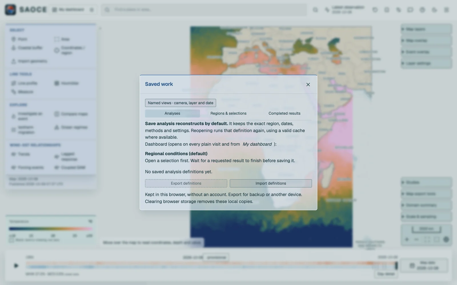
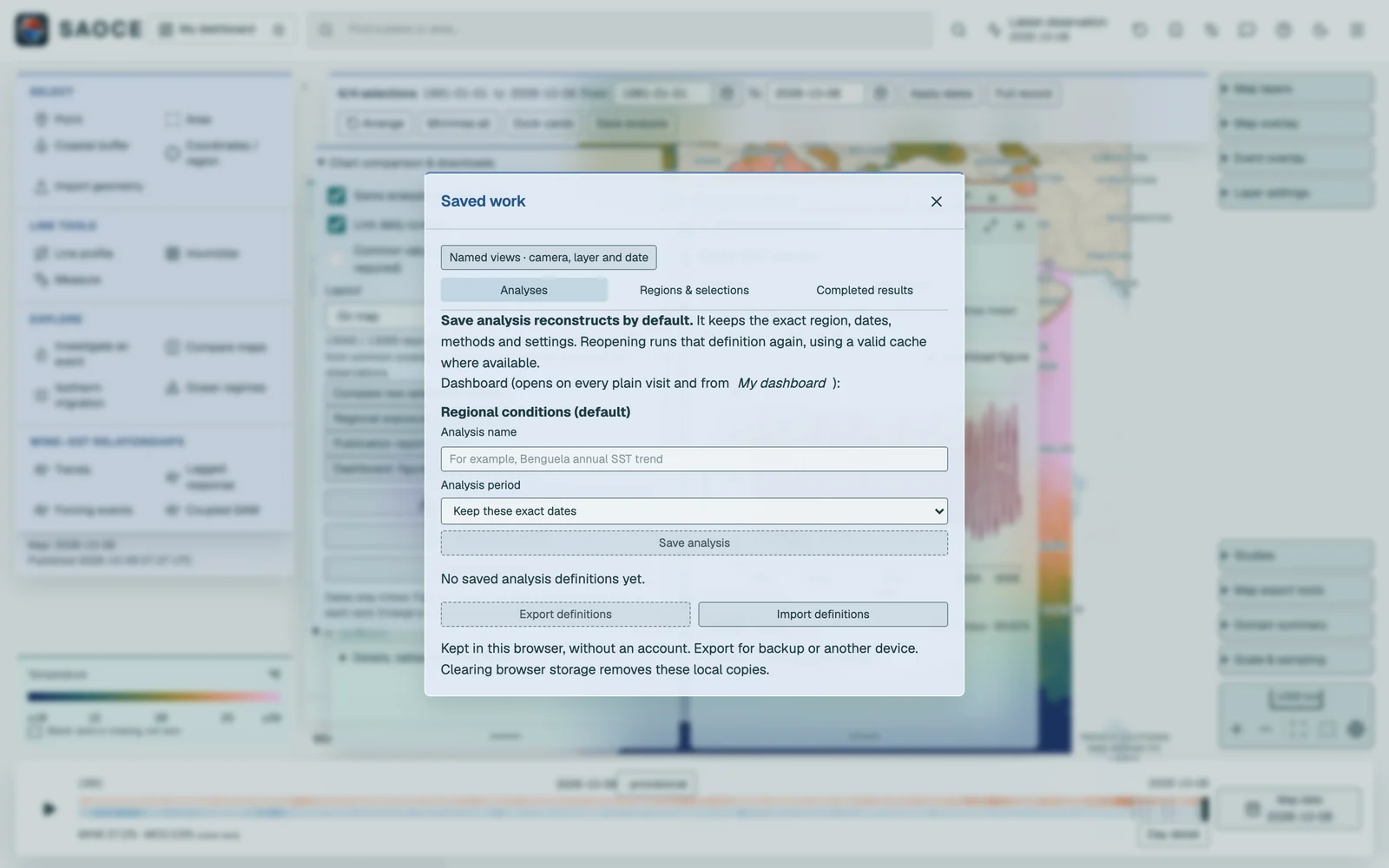
Export definitions creates a portable JSON backup. Import validates the definition before it can be reconstructed. The Regions tab keeps exact reusable geometries independently of analyses, including imported shapefiles. No account is needed. Completed results is a separate tab: Save completed analysis preserves the current figures, numeric tables, definition and provenance, and opening it reads the preserved values without contacting the calculation service. Files carry SHA-256 integrity checks.
The methods behind every exported statistic are documented under Statistical methods.