
Help and methods · 6
Questions and advanced analyses
Every card carries the same menu of methods, grouped under seven questions. Choose the question and the method on the card, change its settings and apply them, and read the outcome sentence; the full figure, the additional figures, the statistics, the data and the methods disclosure open when the card is expanded. The same seven groups organise command search.
One selection, a clear question
A point can use 1, 4 or 16 native pixels. An area uses its exact rectangle, buffer or polygon. The analysis interval is shared by the cards of a group and is independent of the map date. Existing named analyses and share links retain their identifiers. Method settings and complete results travel in their exports.
Choose the question and the method on one row. Costly settings (knots, periods, thresholds, event type and metric) sit under the selector with an Apply button, so a refit never starts from an unfinished edit; a label distinguishes unapplied settings from the completed figure. Choose a figure under Explore this result on an expanded card. Figure layers change the display only. Statistics and uncertainty, Data and coverage, and Methods and provenance open separately below the main figure, and the methods disclosure links to the method’s section under Statistical methods. Unsupported records produce a specific reason rather than a substitute model.
Unless a method states otherwise, complete calendar years or months need at least 90% observed days. Regular-series methods require consecutive eligible periods. Gaps are never interpolated. Every linear regression reports the same slope, standard error, 95% lower and upper limits, whether the interval crosses zero, p-value, R², sample size, degrees of freedom, residual correlation and RMSE.
What are the conditions?
Start with the observed temperature, its departure from the fixed 1991–2020 seasonal baseline, or the usual annual cycle. Missing observations remain gaps.

Seasonal cycle
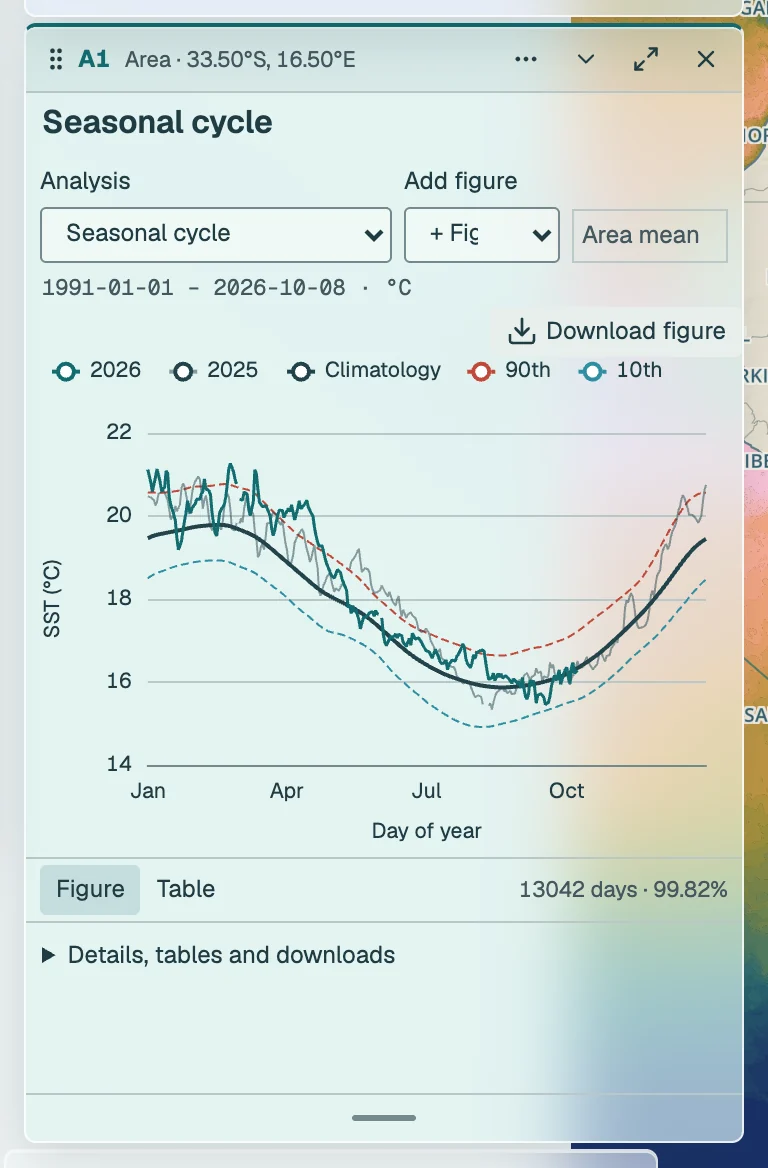
The fixed 1991–2020 seasonal climatology and 10th/90th-percentile thresholds, alongside the latest two calendar years. It keeps its full-record baseline context independently of the analysis interval. Method details
Summary of conditions and change
An overview of a selection: observed mean, median, spread and range; the decadal trend of annual means; the heatwaves and cold-spells of the interval with their three strongest events and the trend of their duration; and whether a single shift in level is detected. Each line is the outcome sentence of the named method, drawn from the same calculations, and opens that method. Method details
Daily SST series
The native OSTIA foundation SST record, with a spherical ocean-cell-area-weighted mean for a region. A daily value requires 90% of its fixed ocean support. Missing days are gaps, not zero. The map date and analysis interval are independent. Method details
SST anomaly series
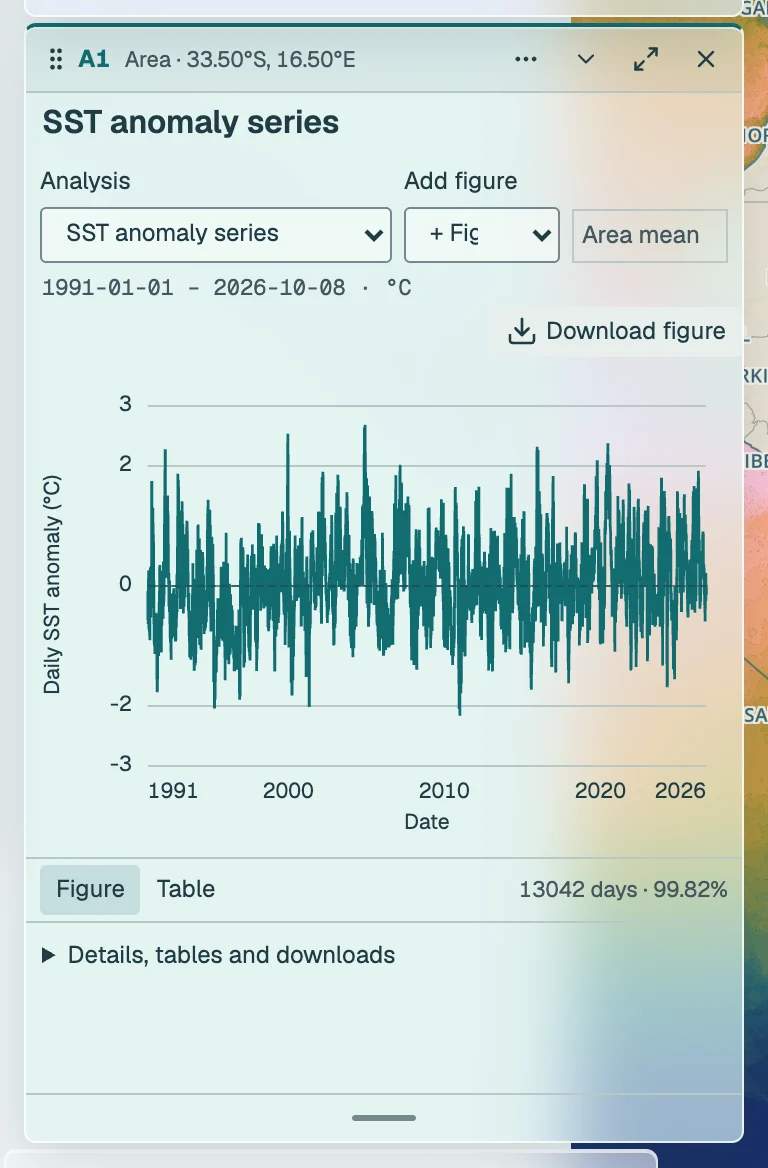
SST minus the pinned heatwave3 day-of-year climatology for 1991–2020, calculated on the same selection. Either missing term makes the anomaly unavailable. The baseline does not change when the displayed interval changes. Method details
Distribution of daily values
The distribution of the selection's daily support-mean SST over the analysis interval: bins of equal width between the observed minimum and maximum, their number the square root of the day count held between 8 and 18, with the mean, median, 10th and 90th percentiles marked. Missing days are left out, never filled. For areas and buffers each day is already the cell-area-weighted mean; the histogram describes time, not space. Method details
Seven-day change
SST on the chosen day minus SST exactly seven calendar days earlier. Both endpoints must be observed. Available in native point or linked rectangle cards. Method details
Uncertainty
The archived pixel standard error. For multiple pixels this is a conservative weighted upper bound assuming perfectly positively correlated errors. The historical archive may contain no uncertainty for a day; temperature availability does not imply uncertainty availability. Method details
How has it changed gradually?
Compare the direction, rate and timing of change. Annual fits use complete calendar years with at least 90% daily coverage. A fitted pattern does not identify its cause.

Decadal SST trend
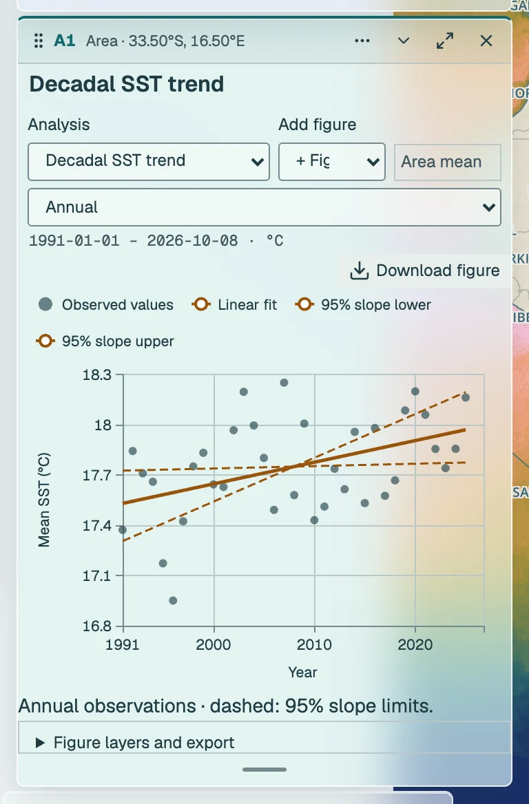
Complete annual, monthly or seasonal period-year means, with at least 90% daily coverage and ten eligible years. The trend estimator pw-gls-ar1-v3 (iterated Prais–Winsten GLS with calendar-gap-aware AR(1) residuals and a bias-corrected ρ, run in R) reports the slope per decade, standard error, lower and upper 95% limits, whether they cross zero, p-value, R², sample size, residual correlation and RMSE. The limits and p-value come from a 499-replicate parametric AR(1) bootstrap-t; the residual degrees of freedom are n − 2 and the effective sample size is reported for orientation only. Method details
Quantile regression (quintile bands)
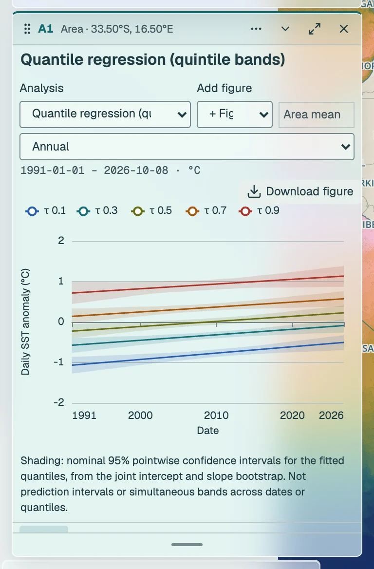
Quantile regression of daily SST anomalies (SST minus the 1991–2020 climatology) on time at τ = 0.1, 0.3, 0.5, 0.7 and 0.9, so the seasonal cycle cannot bias the slopes. Uncertainty is a 499-replicate residual moving-block bootstrap in 365-calendar-day blocks laid on the calendar; the 95% interval is the percentile interval and the sign statement says whether it excludes zero. No p-value is reported and no second AR(1) correction is applied. Ten calendar years are required. Quantile lines may cross. Method details
GAM and periods of warming / cooling
At least 10 complete years. Fits annual means; daily to annual points are display choices.
A cubic-spline GAM fits complete annual SST means with calendar-time AR(1) residuals. Automatic REML chooses smoothness; a nearly straight fit is allowed. Knot-controlled mode removes the roughness penalty for exploratory sensitivity. The mean curve has pointwise 95% bands. Its derivative has a simultaneous band whose critical value is calibrated by a 99-replicate parametric bootstrap from the fitted curve and AR(1) residuals (2,000 joint coefficient draws if too few refits succeed); dated warming or cooling intervals are where that band excludes zero. A knot-sensitivity table repeats the automatic fit at 4, 6, 8 and 10 knots, and a notice appears when whether the band excludes zero anywhere depends on that choice. Changing displayed daily/weekly/monthly/annual points does not refit it. Method details
Robust trend and Mann–Kendall
At least 10 complete years. The slope interval and the annual and like-month rank tests use an AR(1) sieve-bootstrap null.
Theil–Sen is the median pairwise annual slope; its interval and the Mann–Kendall p-value come from an AR(1) sieve bootstrap (1,999 replicates from the residuals about the Theil–Sen line, bias-corrected ρ), and the seasonal test sums S over like months with a matching sieve null. The analytic Hamed–Rao p-value is shown for reference only. The trend estimator pw-gls-ar1-v3 is fitted to the same years for comparison. Theil–Sen resists unusual years; agreement across methods is a sensitivity check, not independent confirmation. Method details
Sensitivity to start and end years
At least 10 complete years per fitted window. Dots are individual, not global, significance.
Every admissible first/last-year pair with at least ten valid complete years is fitted by the trend estimator pw-gls-ar1-v3 with a Student-t interval on n − 2 degrees of freedom. The diamond marks the effective selected interval. Each dot marks an individual 95% slope interval excluding zero; the many overlapping tests are not a global significance test. The table includes the full regression statistics for each fit. Method details
Time of emergence
Needs 27 baseline years and a fitted period containing the baseline centre. No extrapolation.
Compare linear and GAM signals relative to their fitted value at the 1991–2020 baseline-centre year. Noise is the standard deviation of baseline annual means about their 1991–2020 linear fit, so baseline warming is not counted as noise; the raw SD is reported beside it. A signal must exceed one or two baseline SD for at least five consecutive complete years and remain beyond it through the last observed year. Blank means not established. No future extrapolation or emergence-date confidence interval is claimed. Method details
Warming stripes
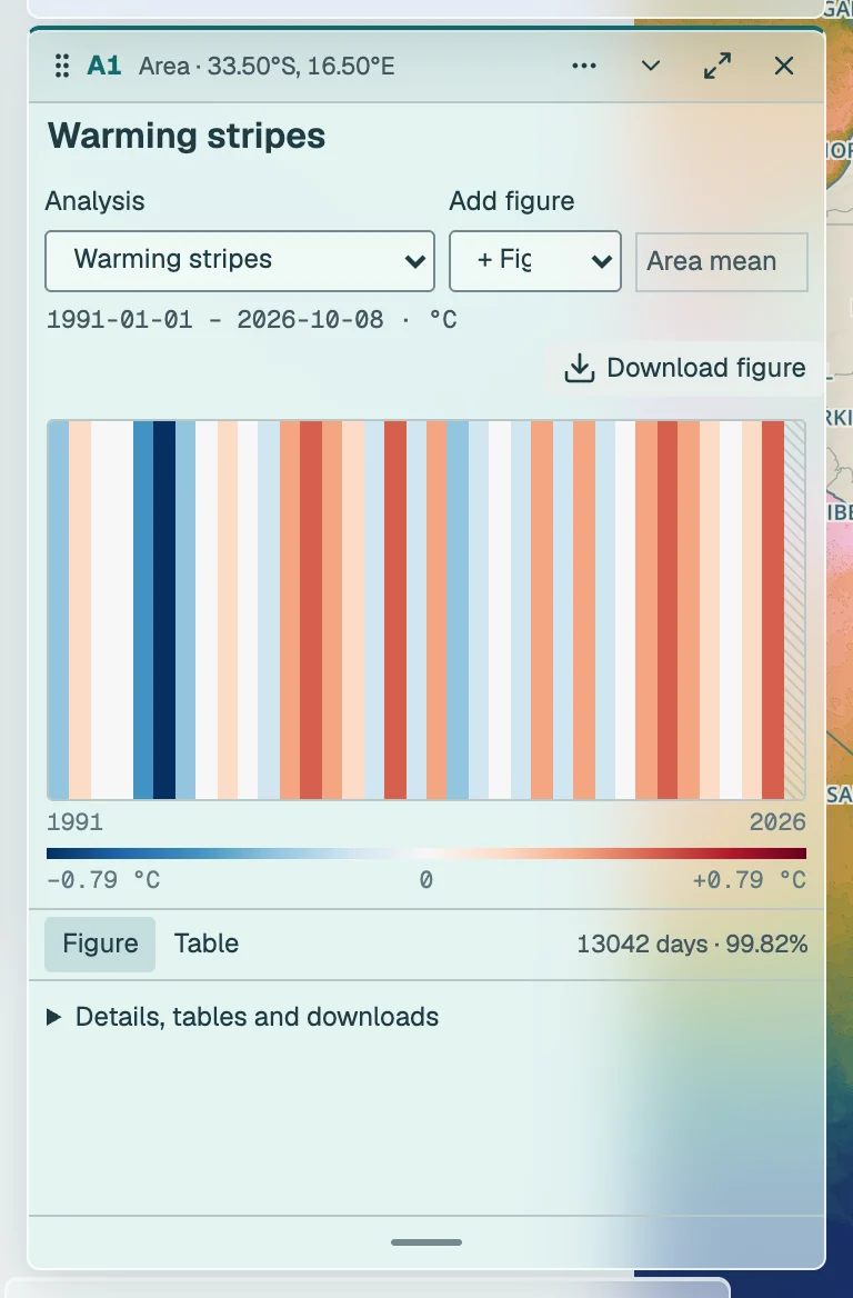
Annual means relative to the 1991–2020 annual-mean baseline, with the colour scale saturating at ±2.6 standard deviations of the 1991–2020 annual anomalies; the baseline and the scale are fixed by the full record, and the displayed years follow the analysis interval. Complete years need 90% coverage; unavailable years are hatched. Method details
Cumulative SST anomaly (CUSUM)
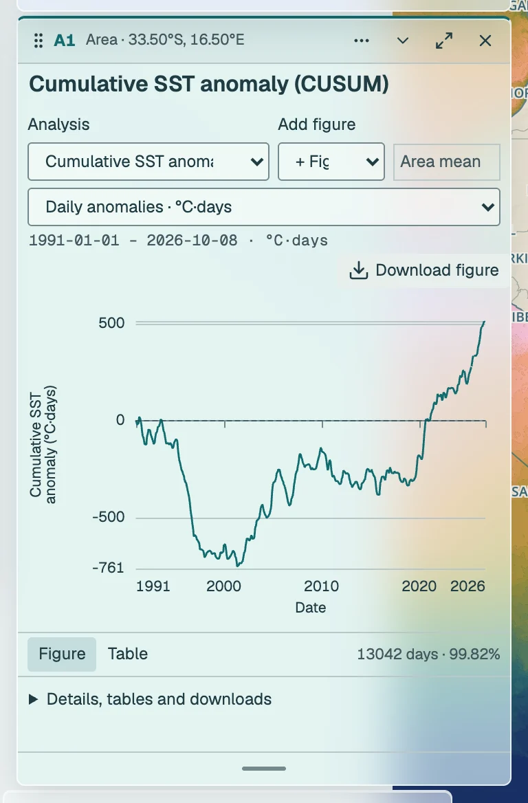
A running sum of anomalies starting at zero at the selected start date. Choose daily °C·days or monthly °C·months. Monthly means require 90% calendar-month coverage. Missing steps stay gaps and add nothing; the sum carries over them. A bend is descriptive, not a changepoint test. Method details
Did it change abruptly?
Test whether levels or slopes changed. A selected breakpoint is a statistical candidate. Correlated variation, endpoint choice and the minimum segment length can affect it.

Multiple shifts in mean or variance (PELT)
At least 20 consecutive annual means; 5 years per segment. Descriptive segmentation in three views, with change-date stability from AR(1) sieve refits, conditional on the step model.
Gaussian PELT on consecutive annual SST means detects mean changes, or mean and variance changes, with fixed MBIC penalty and five-year minimum segments; a change in mean is tested on the series divided by its robust SD because the Gaussian mean cost assumes unit variance. The detector is run in three views (the series, the linearly detrended series and the AR(1)-prewhitened series), because it assumes independent noise. Segment means, SDs, candidate dates and squared-error reduction are reported. Change-date stability refits PELT on 499 AR(1) sieve replicates about the fitted segment means: the share placing a change within two years of each candidate, the range of the nearest refitted change, and how often more or fewer changes are selected. Stability is conditional on the step model; it is not a test against no change. Method details
Single shift (Pettitt)
At least 10 years of daily anomalies, with 5 years on either side of a candidate. Three-year (1,095-day) block null.
The maximum Pettitt rank statistic on observed daily anomalies identifies one candidate date, with at least five years on either side. A 499-replicate moving-block bootstrap in blocks of three calendar years (1,095 days), laid on the calendar with absent days kept absent, calibrates the maximum statistic over the searched dates, so persistence up to three years is in the null. The test is repeated after removing a linear trend in time, because a gradual trend registers as a mid-record shift: a candidate that remains after detrending is a step beyond the trend; one that does not is not distinguishable from persistent variation or a trend. No change-date interval is claimed. Method details
Sequential regime shifts (STARS)
At least 25 consecutive years. Fixed 10-year cut-off; pre-whitened reference STARS.
Rodionov STARS uses the pinned Stirnimann reference implementation, with ten-year cut-off, Huber weight 1, nominal p = 0.05 and MPK pre-whitening with five-year subsamples. Both the original SST regime means and regime-shift index are available. The nominal p is an algorithm setting, not an adjusted shift p-value. Cut-off sensitivity and incomplete recent regimes limit interpretation. Method details
One change in slope
At least 15 consecutive years, 5 per side. Bootstrap intervals are conditional on fitting one break.
A continuous one-break segmented regression on annual means, using the pinned R segmented package. Five observations are required on each side. An AR(1) sieve bootstrap (199 replicates simulated about the fitted stick) refits the breakpoint and both slopes with the same estimator, giving percentile intervals for the break year, each slope and the change in slope. When the break interval covers most of the admissible range the summary says so: the data then do not constrain the break date. These intervals assume a one-break model; they do not establish that a break is needed. Method details
Multiple changes in slope (Bai–Perron)
At least 20 consecutive annual means, 5 per segment. BIC chooses the number of breaks; AR(1) sieve refits report their stability; segment intervals need 10 years.
Bai–Perron least-squares structural breaks use the pinned strucchange implementation. BIC selects the number of breaks, with at least five annual observations per segment. Each segment’s slope comes from the trend estimator pw-gls-ar1-v3; segments of at least ten years carry a Student-t interval conditional on the selected partition, shorter segments an estimate only. Break-date stability repeats the BIC selection on 199 AR(1) sieve replicates about the segment fits and reports how often each break recurs within two years, the range of the nearest refitted break and how often a different number of breaks is chosen. BIC is not a correlation-adjusted significance test. Method details
Is the seasonal cycle shifting?
Compare the timing, size and duration of the annual temperature cycle. Threshold-based seasons depend on the chosen temperature; this never changes the operational 1991–2020 event baseline.

Seasonal amplitude and timing
At least 10 complete years. Two-harmonic annual cycles; trends in amplitude and timing.
Fit two annual harmonics in R to each complete year’s observed daily SST, omitting missing days. Compare peak-to-trough amplitude and unwrapped warmest/coldest phase-day timing with the trend estimator pw-gls-ar1-v3 and its bootstrap-t interval. Phase is day/(365 or 366) of each year and the curve is evaluated on a 365-day grid of equally spaced phase days. Each year’s cycle-fit precision (residual SD and a delta-method amplitude SE) is reported; that first-stage error enters the trend’s residual variance, so the slope interval includes it, with years weighted equally. Near-flat cycles have no timing estimate. Multiple peaks can destabilise timing. Method details
Warm-season onset, end and length
July–June years with 90% coverage. At least 10 observed seasons for a trend.
Within each July–June year, find the longest observed spell of at least five days at or above the chosen absolute threshold, taking the earliest if tied. Report onset and last day as day numbers of the thermal year (1 July = day 1) and length as their difference. Missing days split spells; unobserved adjacent crossings and thermal-year edges censor the relevant date. No-spell years are missing, not zero. At least ten supported seasons are needed for each trend, fitted by the trend estimator pw-gls-ar1-v3 with its bootstrap-t interval. Method details
Compare climatological cycles
Uses the full 1991–2020 baseline and a separate comparison window of at least 20 complete years. The general analysis-period filter does not apply; set comparison years below. Overlap is reported.
Compare 1991–2020 with a user-selected window of at least twenty complete years, defaulting to the latest twenty. Both mean and 10th/90th-percentile day-of-year curves are recomputed with heatwave3::ts2clm3, the production detector's own climatology (11-day pool, 31-day circular smoothing, non-leap 29 February filled from its neighbours before pooling as the detector does). Shared years take the same resampled value in both climatologies. The 199-replicate pointwise intervals resample whole residual years about day-specific linear trends. The operational event baseline is unchanged. Method details
Thermal-envelope explorer
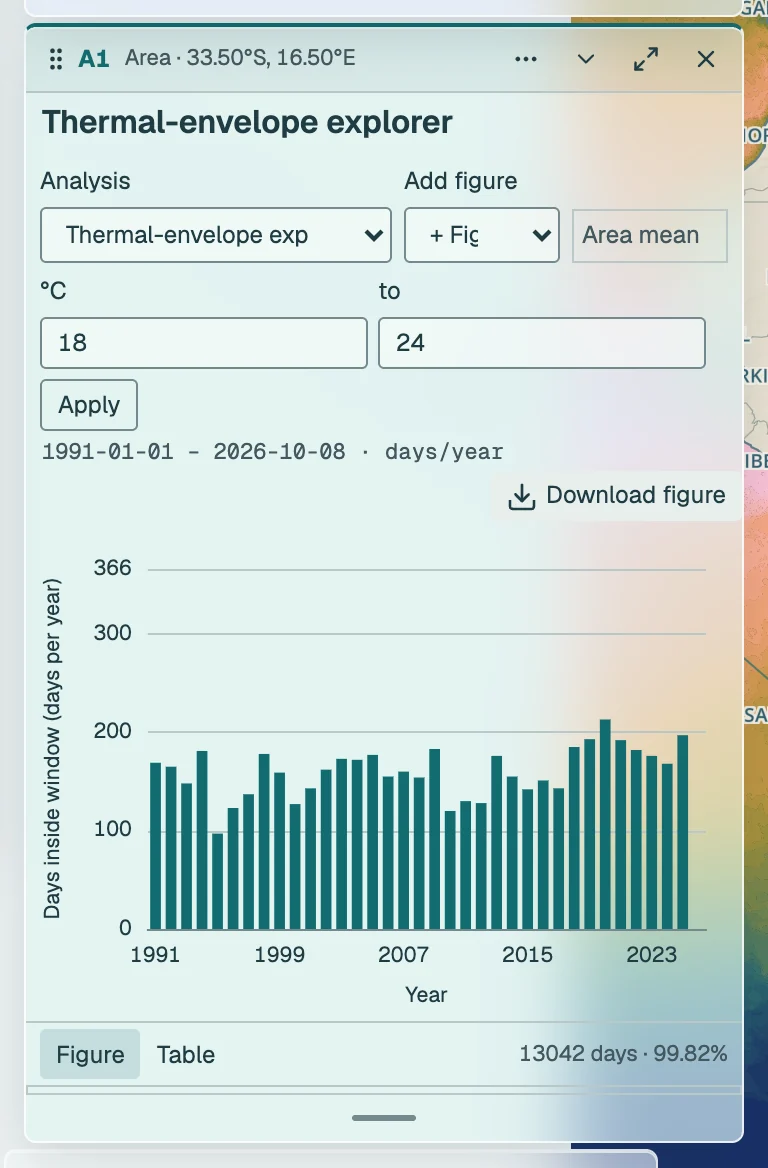
Counts observed days inside inclusive lower and upper absolute-temperature limits. Years below 90% coverage remain missing and are not scaled up. From ten retained years the annual slope comes from the trend estimator pw-gls-ar1-v3 with its bootstrap-t interval and p-value in the common regression report; with fewer years the slope is descriptive OLS without an interval. Display-cell classification on the current map is separate from the regional time series. Method details
Is it becoming more variable or persistent?
Look beyond the mean: spread, memory and recurring periods answer different questions. These analyses use daily anomalies against the fixed seasonal baseline. Missing dates are never interpolated.
Changes in temperature variability
At least 10 complete years of anomalies. Rolling spread needs consecutive 5-year windows.
Compare within-year anomaly SD, variance of adjacent observed-day differences and centred five-year SD of annual means. Daily differences also require 80% of adjacent pairs. All three annual summaries use the trend estimator pw-gls-ar1-v3 with its bootstrap-t interval, with each year’s sampling SE of the SD reported; the overlapping rolling-SD interval is approximate because neighbouring windows share four of five years. Greater spread can be relevant to extremes without establishing a mechanism or cause. Method details
Persistence and decorrelation time
At least 10 complete years of anomalies. Gaps split every daily sequence.
For each complete year, estimate lag-one correlation and the first integer lag where daily-anomaly autocorrelation falls to 1/e. Every pair must have observed intervening days; search at most 90 days, with at least 30 pairs per lag. An unresolved crossing is missing, not zero. Trends use the trend estimator pw-gls-ar1-v3 with its bootstrap-t interval on supported annual summaries; the large-sample SE of each year’s correlation is reported, and that first-stage error enters the trend’s residual variance. Method details
Recurring periods and wavelets
At least 120 complete months spanning 10 years. Wavelet edges and gaps are masked.
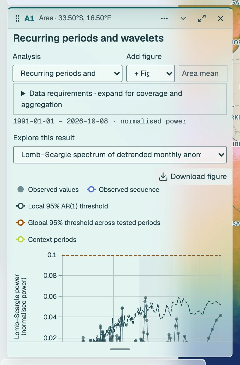
Detrend complete monthly anomaly means in actual calendar time. Lomb–Scargle (lomb::lsp, native frequency grid, periods capped at 20 years and half the record) omits missing months, with 199 AR(1) surrogates retaining the same mask for local and global thresholds. Morlet wavelets (biwavelet::wt, ω₀ = 6, periods capped at 16 years) run separately on uninterrupted sequences; gaps and the cone of influence are masked. Dots mark cells above a global 95% level, the 95th percentile over the same surrogates of the largest power-to-local-threshold ratio inside the cone, so they allow for the search over all times and scales. ENSO (2–7 years), IOD (2–5) and decadal (8–20) labels are overlapping context, not attribution. Method details
Climate-mode context (one index: ENSO, IOD or SAM)
At least 36 months with both a complete monthly SST anomaly and an index value. Lagged Pearson correlation with autocorrelation-adjusted intervals; descriptive context, not attribution.
Monthly SST anomalies (90% daily coverage) against the provider's monthly index at lags from −max to +max months, positive when the index leads. Pearson r per lag; 95% intervals from the Fisher transform with an effective sample size after Bretherton et al. (1999) from both lag-one autocorrelations, each taken over genuinely consecutive months; a Bonferroni threshold across all requested lags. Effective N is capped at the pair count; intervals require N > 3 and three adjacent pairs. Bounds are approximate pointwise intervals, not simultaneous bands. Raw monthly coverage and provider provenance are exported. No causal claim. Method details
How do extremes behave?
Events are detected in the full record. Metric trends assign whole events by peak date. Years without an event are zero for counts and missing for mean event intensity or duration. A regional event is detected in the area-mean SST, not a count of grid-cell events. Area occupancy instead measures the ocean area covered by native-cell event categories.

Marine heatwaves
Full-record marine heatwaves from the pinned heatwave3 detector. The overview and date search select overlapping events, retaining full duration and intensity. Select a peak-date lollipop or an event-list row to open its evolution. Threshold departure is available separately or as an optional overlay; comparison of the three largest metric-magnitude events is explicit. Method details
Marine cold-spells
Full-record marine cold-spells from the pinned detector. Positive plotted threshold exceedance means colder than the cold threshold; intensity metrics retain their recorded signs. Event evolution, filters and monthly/seasonal metric trends follow the same rules as marine heatwaves. Method details
Area occupied by MHWs / MCSs
Area selections only. Daily percentages need 90% observed ocean-area coverage. Trends need ten consecutive complete, stable years with 90% valid days each. Category I–IV occupancy differs from events in area-mean SST.
Native-cell MHW or MCS categories within the selected ocean area. Any is the sum of exact categories I–IV; category-zero joined gaps are excluded. Rectangles use fractional spherical cell overlaps; polygons retain holes and use whole cells whose centres lie inside. Daily percentages use observed ocean area and require 90% coverage of fixed first-day ocean support. Annual means need 90% valid days; trends need ten consecutive complete stable years and exclude the final seven provisional event days. The trend estimator pw-gls-ar1-v3 reports percentage points per decade with individual bootstrap-t 95% intervals. This measures spatial occupancy, separately from events in the region’s mean SST. Method details
Rapid extreme thermal transitions
Area selections only. Last MHW day to first MCS day, or vice versa, in the same native cell within n days. Requires continuous observed data across the look-back window. Descriptive fixed-cell metrics for an unpublished concept. Endpoint-category filters keep the original pair. Fixed-interval rate windows are independent of the maximum transition interval.
Descriptive fixed-cell suite for AJ Smit’s unpublished concept: last categorised MHW day to first subsequent MCS day, or vice versa, within 1–90 elapsed days (default 7), requiring continuous observed SST and both category archives. Both original endpoints must reach the chosen minimum category I–IV; their dates never move to stronger days. Arrival dates select transitions. Results include counts, unique affected area, area-weighted elapsed time, raw/anomaly changes and rates, observed arrival-aligned trajectories, and separate complete/censored endpoint persistence. Anomalies use the same-cell approved 1991–2020 seasonal mean. Arrival persistence follows up to 30 days. Sensitivity uses common fully observed 90-day histories. A separate 1–90-day interval gives warming/cooling rates for all observed SST windows, including non-events. Every diagnostic retains its observation support. The final seven source days are provisional. No moving-patch tracking, severity score or inference. A disclosed 20,000-row catalogue cap never limits aggregates. Method details
Trends in event metrics
At least 10 valid period-years. Choose a month, season or full year; no-event means stay missing.
Fit annual means of complete detected-event metrics, assigning events by their peak date within an annual, calendar-month or seasonal period. December belongs to the following DJF year. A period needs 90% source coverage, and at least ten valid period-years are needed for a slope from the trend estimator pw-gls-ar1-v3 with its bootstrap-t interval. No-event means remain missing. All twenty metrics and both event types use the same regression report and full-record detection. Method details
Trends in event counts or days
At least 10 consecutive complete years for the estimate, 20 for an interval and p-value. Exposure-adjusted Poisson fit with 1,999 block-pairs bootstrap resamples; NB2 reported when overdispersed.
Retain adequate zero-event years. Counts are assigned by peak year; event days use the detector’s daily flags. The estimate is the log-link Poisson slope with an offset for observed days / 365.25; Pearson dispersion above 1.5 selects an NB2 fit as the dispersion diagnostic. Uncertainty comes from a block-pairs bootstrap-t: whole year rows are resampled in three-year moving blocks and the slope refitted 1,999 times, with a Student-t multiple of the bootstrap SE on block degrees of freedom. The interval and p-value are reported only from 20 complete years, the range in which the method is calibrated; with ten to nineteen years the rate ratio is an estimate only. Rate ratios use 1 as no change. Day counts are bounded by coverage, so the log-link approximation needs care near saturation. Method details
Accumulated heat stress (DHW map)
Degree heating weeks summarise accumulated heat stress on the map. They describe the temperature product and its fixed baseline; they are not a direct observation of coral damage. Method details
What was the wind?
ERA5 reanalysis 10 m wind over the South African box (11–38.5°E, 40–22°S), 1991 onward, against its 1991–2020 day-of-year climatology. Stress uses the Large and Pond (1981) bulk formula on hourly wind; curl is least reliable within a cell or two of the coast. The wind reaches the tracker about five days behind real time. Place a wind figure under an SST figure to read the two together; a lagged relationship is a description, not attribution.

Wind rose (ERA5)
Daily wind speed (ERA5)
Daily wind stress (ERA5)
Daily wind stress curl (ERA5)
Wind speed trend (ERA5)
Wind stress trend (ERA5)
Wind stress curl trend (ERA5)
How do two selections compare?
Keep the spatial support, years and method explicit. Paired slope differences use common years and retain the dependence between selections. Comparing periods answers a different question from comparing slopes.

Compare two time periods
Two non-overlapping periods, each with at least 10 complete years. Percentiles describe annual means.
Compare two non-overlapping periods with at least ten complete annual means each. Report the mean and 10th/50th/90th-percentile differences (B minus A). These percentiles describe annual means, not daily extremes. The mean difference carries an approximate AR(1)-effective-size Welch interval; every difference carries a p-value from a 1,999-replicate AR(1) sieve bootstrap under the null of no difference. Separate periods are assumed independent, and simultaneous testing is not corrected. Method details
Compare two selections’ trends
Two selections and at least 10 common complete years. Difference is B minus A.
Fit the paired difference B minus A on the common complete years with the trend estimator pw-gls-ar1-v3 and its bootstrap-t interval, which retains cross-selection covariance and annual serial dependence. The separate slopes of A and B are shown for comparison; the paired slope need not equal their difference because each series carries its own AR(1) estimate. Identical series have zero difference. Use Chart comparison & downloads in a group with two linked selections. Method details
Compare areas side by side
Two exact drawn rectangles share analysis, dates and method settings. Each series keeps its own area weights and coverage. Side-by-side fits alone do not test a difference; use Compare two selections’ trends for that statistic. Method details
Compare maps and dates
Split two fields on one camera: dates, layers or the selected day’s 1991–2020 climatology. This is a spatial display, not a test of a temporal trend. Method details
Other card figures
Each method draws its own figure on the compact card, with titled axes and units, and the same figure at full width when the card is expanded.

Every method, with its data, estimator, uncertainty, requirements and references, is documented under Statistical methods.