
Help and methods
Overview and workflow
SAOCE shows daily sea surface temperature (SST), its departures from the 1991–2020 normal, and the marine heatwaves (MHWs) and marine cold-spells (MCSs) detected from it, across the seven African Large Marine Ecosystems, within 26°W–60°E and 50°S–51°N. These pages describe every control in the interface and the statistics behind each result, so that a reader can reproduce what the map reports.
Read NEWS for brief daily bug fixes, changes, improvements and new features. SAOCE remains under active development and testing; performance is limited by the current server while a production move is pending.
What the interface does
The map is the entry point. Layers → Product and layer settings chooses the SST product, OSTIA or OISST. A data layer chooses the field: daily SST, the SST anomaly, a long-term trend, a seven-day change, the analysis uncertainty, the SST gradient, accumulated heat stress, or an event category map. The timeline chooses the day. Every analysis then starts from a selection on that map and opens as a card in the right-hand column. A plain visit opens your dashboard first: one docked Benguela seasonal-cycle example, or the analysis you saved as home. The workspace holds up to four selections of any kind at once (points of 1, 4 or 16 native pixels, rectangles, coastal buffers, named reporting regions and your own shapefiles), keeps completed work while you explore, and separately holds up to four Hovmöller sections. It also adds the line tools, isotherm migration, saved studies and the publication report.
Every card carries the full menu of methods, grouped by seven questions: what the conditions are, how they changed gradually, whether they changed abruptly, whether the seasonal cycle is shifting, whether variability or persistence is changing, how extremes behave, and how two selections compare. Each result opens with one sentence stating the finding and its uncertainty, and the card’s Graph options menu exports the plotted data as CSV, netCDF or JSON and the figure as SVG or PNG.
Three rules hold throughout. Source-absent days are shown as gaps and are never interpolated or filled. The climatological baseline is fixed at 1991–2020 and is computed from the selected product’s own record; OSTIA uses reprocessed data only. Event detection runs in one place, the pinned heatwave3 R package, with fixed parameters that the interface cannot change.
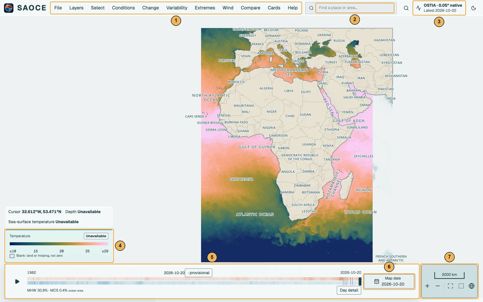
- 1Menu bar: File, Layers, Select, the six analysis questions, Cards and Help.
- 2Place search: locates a place or reporting area without creating a selection.
- 3Latest observation: the newest published day; opens the Data status sheet.
- 4The legend at the foot of the left column, with the cursor readout above it.
- 5Timeline: the archive with its heatwave and cold-spell ribbons; drag to preview a date.
- 6Map date: the archive calendar, with Day detail beside it.
- 7Map navigation: scale, zoom and the three framings, at the right end of the dock.
A typical workflow
- Choose a layer and a day. Open the Layers menu and pick a layer; drag the timeline or open Map date for the archive calendar. See Map layers and Data, dates and status.
- Select the place of interest. Choose Point, Area or Coastal buffer from the Select menu and click the map, or choose Coordinates / region to type coordinates, choose a reporting region, pick a saved region or load a shapefile. See Selection tools.
- Choose a question and a method. New point, area and buffer selections open on Seasonal cycle. Summary of conditions and change follows it in the menu, which groups every method under the seven questions. Change the method, the pixel support or the shared analysis interval and the card recalculates. See Questions and advanced analyses and Statistical methods.
- Read the result. The outcome sentence states the estimate with its 95% interval and the method’s standing caveat. Scroll within the card for its settings, statistics, source tables and methods. Expand the labelled disclosures to read those details; the methods disclosure links to the relevant section of these pages. The arrows in the header give the floating card more figure space.
- Keep it. Use the card’s Graph options to export the plotted data or the figure, Publication report (PDF) for a report of ticked results, Save analysis to store the definition for later reconstruction, or a link that replays the view. See Comparing, exporting, sharing and saving.
Contact the maintainer
Report a problem, suggest an improvement or ask a question through SAOCE feedback on GitHub. Reports are public and need a GitHub account. For private feedback or help without an account, email the project maintainer.
Usage and privacy
SAOCE records page visits and selected tool actions, a random browser ID that expires after 35 days, a visit ID renewed after 30 minutes without recorded activity, estimated active viewing time, the server-observed IP address and an approximate country. These private operations records help us understand which features are used, how often browsers return and how usage relates to worker CPU load. Active time is measured while the page is visible and pauses two minutes after the last interaction. Interaction contents and mouse movements are not stored. They are retained for 35 days; expired records are removed when the log is accessed. They do not contain saved names, uploaded geometry, cursor coordinates or URL query strings. A visit or IP address does not identify a person. Browsers requesting Do Not Track or Global Privacy Control do not send these usage records. Country lookup uses an offline database: IP Geolocation by DB-IP. Visitor addresses are not sent to a geolocation service.