
Help and methods · 5
Selection tools
An analysis begins with a selection, and every selection is one linked card carrying the complete method menu, so every statistical method applies equally to a point, a rectangle, a coastal buffer, a reporting region and a shapefile polygon. Up to four selections of any mix can be open at once, whether started from the Start tasks or the selection tools, and each card can carry up to three figures. Lines and sections follow under Profiles, sections and points.
Point
- Press Point under Select and click an ocean or supported lake point. Each click adds a card, up to four.
- Choose 1, 4 or 16 native pixels (0.05° OSTIA or 0.25° OISST) in the card’s support selector, displayed as a fixed 1×1, 2×2 or 4×4 footprint on the map.
The value is the spherical-cell-area-weighted mean of the footprint’s water cells, reported only when at least 90% of the fixed water area is present on the day. Land and missing cells are never replaced by a different ocean location. For several pixels the uncertainty line is a conservative upper bound formed from the weighted source standard errors under perfect positive correlation.
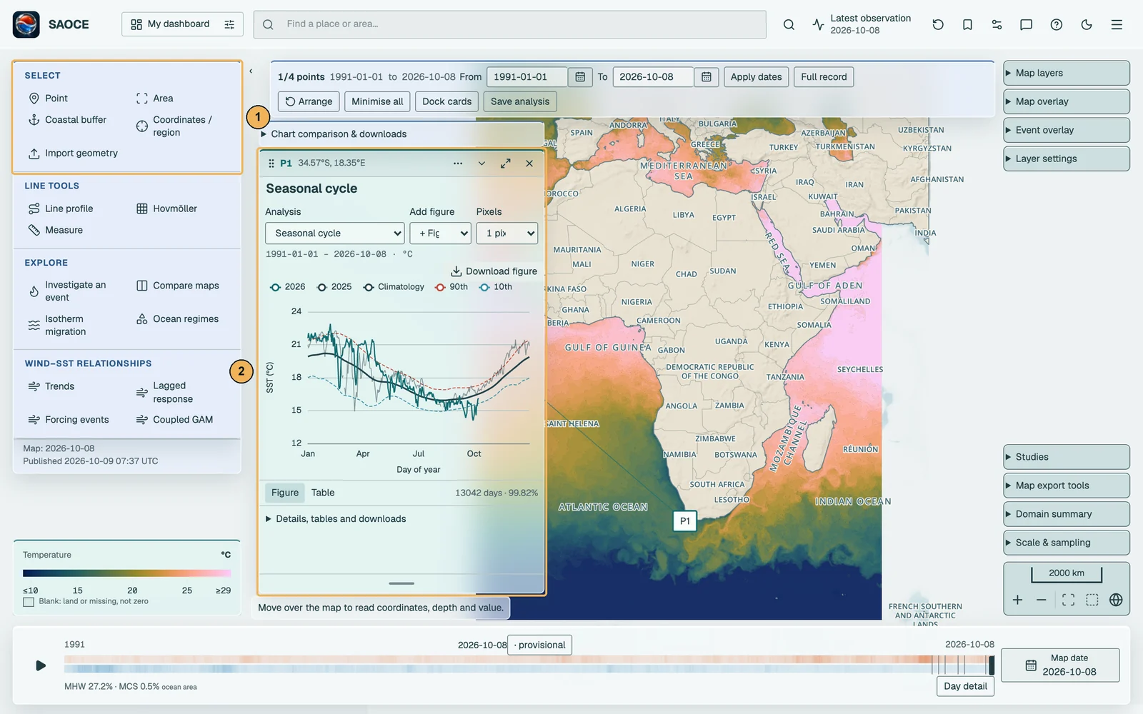
- 1The Select group, with Point active.
- 2The card, linked to its marker.
African lakes
With OSTIA selected, you can view and analyse surface temperatures in Lake Victoria, Lake Tanganyika and Lake Malawi. Choose Point and click within a lake, or draw an Area over part of it. Lake shorelines and names help you locate the water; the native OSTIA cells determine which observations enter the analysis. Plain land, ice and missing observations are excluded. These are lake surface temperatures, although the shared charts retain their SST label. Lake coverage is not added to OISST.
Area
- Press Area under Select. The status bar reads Select the first corner.
- Click the first corner on the map, then the opposite corner. There is no drag.
- The rectangle is outlined and its card opens on the seasonal cycle of its area-weighted series; choose any method from the card’s menu.
Both corners must lie inside the domain and differ by at least 0.05° in both longitude and latitude. This is the geometry-entry minimum; eligible cells still depend on the selected product’s native grid. Escape cancels a selection in progress.

- 1Header: identifier, extent, graph options, collapse, expand and close.
- 2Method and pixel-support selectors.
- 3Figure or Table, and the observed days with their coverage.
Coastal buffer
- Press Coastal buffer and click the start and the end of a stretch of coast.
- In the dialogue, the two clicked endpoints are shown as editable latitude and longitude fields: keep them, or type a published extent exactly, in decimal degrees, degrees and minutes (7 30 S) or degrees, minutes and seconds. Set the offshore distance in kilometres, from 5 to 500 in steps of 5, with 50 as the default, and press Build buffer.
- The buffer polygon is drawn and its card opens on Seasonal cycle, labelled with the length of coast and the offshore width.

Each endpoint, clicked or typed, is snapped to the nearest point on the Natural Earth 1:50 m coastline, the same line the map draws, so a typed latitude fixes the buffer’s meridional extent exactly; a click more than 100 km from any coast is refused. Both points must fall on the same continuous coastline, so an island is a separate coast, and on a closed coastline the shorter way round is taken. The coast between the two points must be at least 10 km long. That segment is buffered by the chosen distance in an azimuthal-equidistant projection centred on it, with flat ends and rounded joins, clipped to the domain; if clipping splits the polygon only the largest piece is kept. The buffer extends on both sides of the line, but land cells carry no values, so the series is an average over the ocean cells inside it.

Coordinates, reporting regions, saved regions and shapefiles
Coordinates / region opens one dialogue with three sources. Your saved regions lists the polygons, buffers and rectangles saved in this browser, including shapefiles you have imported; choosing one analyses its exact geometry. Load a shapefile or GeoJSON… opens the importer, which accepts a zipped ESRI shapefile (.shp, .shx, .dbf and .prj, in any coordinate system, reprojected with the .prj) or WGS84 GeoJSON and WKT, validates it without repair, clipping or simplification, previews it, and saves it under a name for reuse; multipart shapes become separately named parts. Named reporting area lists the seven reporting regions. Otherwise choose the analysis tool and type the coordinates in decimal degrees, east positive and south negative.
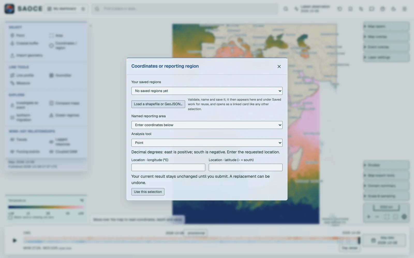
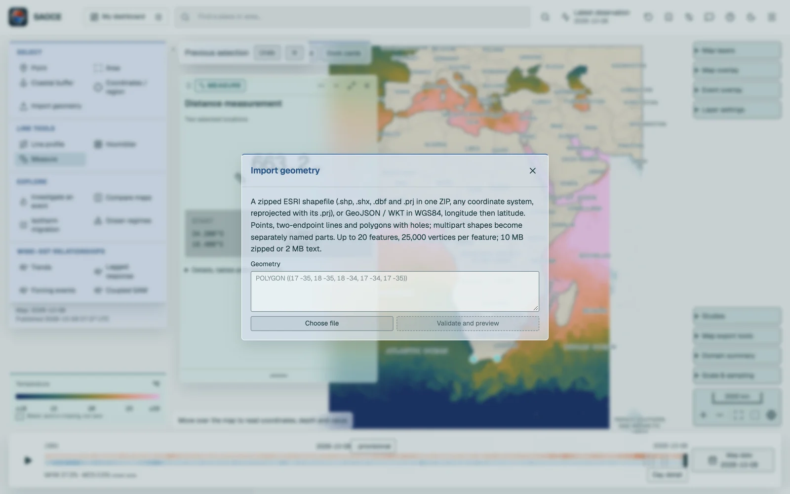
The reporting regions are the Southern African domain, the Benguela, Agulhas, Mozambique Channel and Southwest Indian Ocean boxes, and the Benguela Current and Agulhas Current Large Marine Ecosystems (LMEs). Choosing one opens a card for that region and, for the two LMEs, uses the full Marine Regions polygon including its holes. The boxes are aggregation units for reporting; they are neither ecoregions nor jurisdictions, they may overlap, and values must not be summed across them.
Hovmöller sections have a separate allowance of four cards. They keep their own dates, routes and SST product while sharing Arrange and Dock with selection cards.
Up to four selections
Every card in the group shares the analysis interval and, unless independent analyses are enabled, the method and its settings, so a Benguela rectangle, an Agulhas buffer, a point and an LME can be read side by side. The group toolbar sets the interval, arranges, minimises or docks the cards, and opens Chart comparison & downloads, where Compare two selections’ trends fits the difference of slopes between any two cards with an interval that keeps their shared variability, and Publication report (PDF) collects ticked results.

- 1Group toolbar: analysis interval, arrangement and saving.
- 2A card; each is linked to its marker on the map.
Saved regions and analyses
Saved work in the header stores complete analysis definitions, including the selections, their exact geometry, the methods and settings, and reconstructs them on reopening; its Regions tab keeps reusable geometries independently of analyses. Export and import move these definitions between browsers. See Saving and reconstruction.
How an area becomes a series
Every area selection ends in the same request: the daily area-weighted mean of SST over the cells the area covers, from the first archive day to the last. Two weighting rules apply.
- Rectangles. Cell edges are the midpoints between cell centres. Each cell is weighted by its exact spherical overlap with the rectangle, so a cell cut by the boundary contributes in proportion to the part inside.
- Polygons (coastal buffers, the two LMEs and imported shapes). A cell counts, with its whole spherical area, when its centre lies inside the polygon; holes are excluded. A polygon that contains no cell centre is rejected.
SST_area(d) = Σ w_i · SST_i(d) / Σ w_i over cells with a finite value and w_i > 0
The valid ocean area, i.e. the sum of the weights of the cells that had values, is reported for every day, and the requested area of a rectangle is its spherical area including land. A day with no source file and a day whose cells are all land or missing both carry a null value and nothing is substituted. The expanded card’s methods disclosure states the extent, the ocean cells and area, the number of source days among the calendar days, and the aggregation rule used.