
Help and methods · 4
Map layers
The Map layers picker offers nine SST layers, and switching between them keeps the current map view. Seven are continuous fields drawn with fixed colour limits; two are category maps of detected events. The legend fixed at the bottom left states the limits, the units and the treatment of missing values, the Domain summary reports domain-wide statistics of the displayed layer, and an event overlay can be drawn over the temperature and anomaly fields.
| Layer | Field | Units | Colour limits | Dates |
|---|---|---|---|---|
| Temperature | Analysed foundation SST | °C | 10 to 29 | Any archive day |
| SST anomaly | Daily SST minus the 1991–2020 day-of-year climatology | °C | −5 to +5 | Any archive day |
| SST trend | Rate of change of annual means, GLS with AR(1) residuals | °C decade⁻¹ | −0.6 to +0.6 | A period of complete years |
| 7-day change | Latest day minus the day seven days earlier | °C | −3 to +3 | Fixed to the latest release |
| Uncertainty | Selected product’s analysis error | °C | 0 to 0.8 | The eight days of the release |
| SST gradient | Magnitude of the horizontal SST gradient | °C km⁻¹ | 0 to 0.2 | Served map dates |
| Degree Heating Weeks | Accumulated heat stress over 84 days | °C-weeks | 0 to 16 | Served map dates |
| MHW category | Marine heatwave category where an event is active | I to IV | Categorical | The analysed archive; historical maps on demand |
| MCS category | Marine cold-spell category where an event is active | I to IV | Categorical | The analysed archive; historical maps on demand |
Values below or above the limits take the end colours, and the end ticks of each legend carry ≤ and ≥ to say so. Uncoloured cells are land or cells without a source value; they are never zero. In Layer settings the temperature layer offers the Crameri palettes Batlow, Glasgow, Lipari, Navia and Imola, and the diverging layers share one choice among Vik, Roma, Broc, Bam and Berlin. The chosen palettes also colour the Hovmöller diagrams, the legends and the exported images. Stretch to the visible range rescales the temperature or anomaly colours to the values in view; the legend states the resulting limits, the setting is display only, and exports keep the fixed scientific limits.
Basemap and relief
Land carries a shaded relief from ETOPO 2022 above a flat fill, with quiet country borders and the coast drawn from the same land mask. The sea floor is tinted by depth wherever no data raster covers it: data layers are opaque, so the tint shows only outside the published domain, or everywhere when Show the data layer under Layer settings is switched off to read the bathymetry alone. Depth contours in Map overlays draw over any data layer at a chosen spacing: Low (200, 1,000 and 2,000 m), Medium (seven levels from 100 to 4,000 m) or Dense (nineteen levels from 50 to 5,000 m), all from GEBCO 2026. The relief and contours are context only, never a basis for navigation.
Rivers and estuaries
In Setup → Rivers and estuaries, switch Show rivers and estuaries on or off. This preference is saved automatically in this browser and survives Reset. Major rivers appear at continental scales; zoom in for smaller rivers, coastal water bodies and streams. The map now permits zooming to level 16, beyond the previous limit of 9. Streams enter the source tiles from level 13.
As in Copernicus Marine’s MyOcean viewer, rivers and coastal water bodies provide geographic context at progressively finer scales. SAOCE uses the public GloFASMajor Rivers map for the continental overview. This is a static river network, not a river discharge or flood forecast. It fades into detailed waterways between zoom levels 8 and 9.
Detailed OpenFreeMap tiles use the OpenMapTiles water and waterway layers from OpenStreetMap. Solid blue lines show mapped waterways; dashed lines indicate intermittent flow. Blue areas show rivers, lakes and mapped coastal lagoons. Fine shoreline outlines trace tidal inlets and open river mouths, including those mapped as part of the ocean. Names appear where supplied, and small unnamed features are retained. The outline leaves the SST colours visible; it does not imply that SST observations resolve the inlet.
In South Africa, a turquoise overlay adds the SANBI National Biodiversity Assessment 2018 estuarine ecosystem map, served by DFFE’s public mapping service. It includes small estuaries, micro-systems and associated estuarine shores, without a minimum-area filter. These are mapped ecosystem extents, not today’s wetted area. This older inventory should not be mistaken for the NBA 2025 assessment.
Coverage varies across Africa. This is geographic context, not a complete surveyed estuary inventory or an estuarine habitat classification. A river mouth is not automatically classified as an estuary, and an absent feature is not evidence that none exists. Small or temporarily closed systems can be missing. The overlay does not alter the SST grid, ocean mask or coastal-buffer calculations.
Tiles load only while the overlay is enabled and only for the area and zoom in view. Hiding it removes the tile source. OpenStreetMap data are licensed under the Open Database Licence; attribution remains on the map. OpenFreeMap availability is independent of the SAOCE worker.
Tide gauge stations
Enable Tide gauges in Map overlays, or Tide gauge stations (Research Quality) in Setup. Gold station markers show historical coastal observation sites. Select a marker, or open Station records and choose a station, to inspect its record. Station dates are independent of the SST map date. Setup can save this layer as a default, and named map views preserve its visibility.
Long-term relative sea-level slopes use unflagged, datum-controlled PSMSL RLR annual means with at least 70% coverage over 30 years. Each slope in mm/year comes from the shared Prais–Winsten GLS AR(1) annual-trend estimator with a bootstrap-t 95% interval and p-value; the nodal cycle and the inverse barometer are uncorrected, land motion is included and no projection is claimed. Stations with quality flags or insufficient support show a withholding reason. Under these gates only 3 of 28 PSMSL stations receive a slope, none of them South African, and 7 of 49 Durban hourly years pass the extremes gates, so the absence of a slope is not evidence of absence of change.
Extreme water levels use UHSLC Research Quality hourly records. Documented replaced/questionable days are excluded; years require 90% accepted hourly coverage and 80% in every month. Storm-surge indicators require an additional held-out tidal-prediction check. Event traces distinguish observed water level, fitted tide and non-tidal residual; complete tidal cycles also provide skew surges. These are historical indicators, and weather evidence is needed to identify a storm. Local gauge datums, hourly sampling, source QA reports and gaps remain explicit. Download annual tables and event traces as CSV, or the complete analysis as JSON.
Temperature
The daily analysed SST. OSTIA is a foundation SST, namely the temperature free of diurnal warming, so it is comparable across the day. The domain summary reports the map-domain mean, the observed range and the median analysis uncertainty for the displayed day.

- 1Legend with the fixed 10 to 29 °C limits; Event overlay and Layer settings open from the Layers menu.
Wind (ERA5)
Seven wind layers come from the ERA5 reanalysis (decision record 0015), on a 0.25° grid over the South African coast box, 11 to 38.5°E and 40 to 22°S, from January 1991; outside the box the layer is empty. ERA5 is a model analysis constrained by observations, not an observation, and every wind layer says so. Each day is the 24 hours from 00:00 to 23:00 UTC. Wind speed is the daily mean of the hourly speeds; Wind direction is the direction the daily vector-mean wind blows from, degrees clockwise from north on a cyclic colour scale, so a southerly reads 180°; Wind stress is the daily mean of the hourly bulk stress (Large and Pond 1981 drag law on the 10 m wind), in mN/m²; Stress curl is the curl of the daily mean stress, negative where cyclonic in the Southern Hemisphere, in units of 10⁻⁷ N/m³. The three anomaly layers subtract the 1991–2020 day-of-year mean from the pinned R climatology. All fields are drawn as their native cells over ocean cells only, and direction is never interpolated.
On a wind layer the calendar and timeline run over the whole wind archive, from January 1991 to the latest held day. ERA5T reaches the store about five days behind real time; the days after its release are held as interim wind from the ECMWF IFS open data (the 00 and 12 UTC analyses and their 3, 6 and 9 hour forecasts, eight samples a day), so wind runs about a day behind real time. ERA5T replaces each interim day on release, and every reading, legend and export names the stream. Hovering a wind layer previews that cell’s last 14 days against its 1991–2020 climatology and 10th and 90th percentiles; a map click reads the cell. Under What was the wind? on any analysis card, a wind rose (sixteen sectors from which the daily vector-mean wind blows, stacked by the class of the daily scalar-mean speed, the same speed as the Wind speed layer and series, with calm days below 0.5 m/s of that speed counted apart and the stated mean the scalar mean; an area pools its ocean cell-days with area weights; a period selector confines it to one month or season of every year) or the daily wind speed, stress or stress curl of the card’s point or area is drawn with the same climatology band, so wind can sit under an SST figure for the same place and dates.
Every wind layer carries the arrows of the daily vector-mean wind over its coloured cells. Under the top-right Map overlay dropdown, Wind vectors (ERA5) draws the same arrows above any other layer, SST included: arrows point downwind, their length grows with the vector-mean speed (the magnitude of the day’s mean vector, at most the scalar-mean speed of the Wind speed layer), and they thin with zoom from one per 2° to one per native 0.25° cell. The wind key sits beside the SST legend and both use the displayed map date. If SST is newer than the wind release, an explicit latest-wind-date button moves the map to a shared date. Vectors pause during Compare maps. Hovering a wind layer reads the cell value and, where a climatology exists, the day-of-year mean and the 10th and 90th percentile thresholds. Recent days can be interim IFS or preliminary ERA5T, and the legend and arrows say so; final values replace them, the interim days within about five days and the preliminary months two to three months later. Curl within a cell or two of the coast is the least reliable field, because the model’s coastal cells mix land and sea roughness; wind trends from a reanalysis mix real change with changes in the observing system.
Event overlay
On the Temperature and SST anomaly layers, the Event overlay panel (Layers → Event overlay) draws the heatwave or cold-spell category map of the same date over the field, with an opacity slider and its own category legend. Transparent areas include no event, land and missing data. The overlay is suspended on the other layers and in Compare maps, and it is included in map image exports with its legend.

- 1Category map choice and opacity.
- 2The overlay's own legend for the same date.
SST anomaly
The anomaly is the day’s SST minus the climatological mean for that day of the year, cell by cell. The climatology is the heatwave3 seasonal climatology for 1991–2020, the same field that defines the event thresholds, so a map anomaly and a regional event refer to the same normal. The domain summary reports the area-weighted domain anomaly and the observed anomaly range.
anomaly(x, y, d) = SST(x, y, d) − climatology(x, y, day-of-year(d))
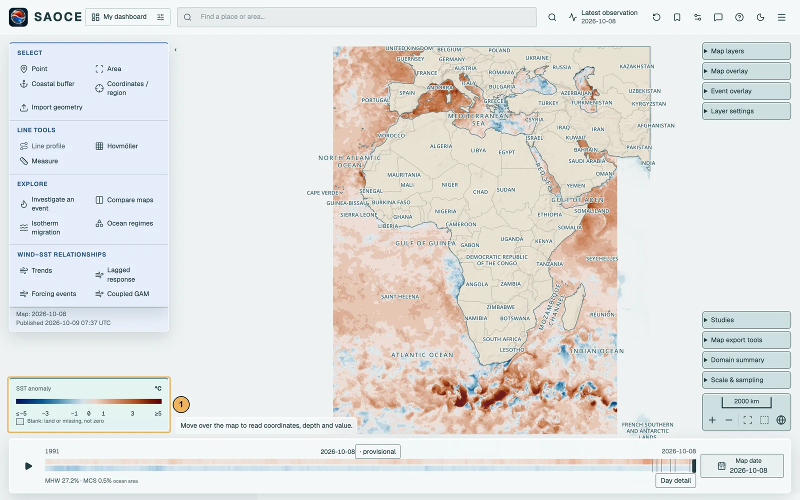
- 1Diverging legend, −5 to +5 °C.
SST trend
The trend layer fits a straight line to the annual mean SST of every cell over a chosen period of complete calendar years. An annual mean is computed only where at least 90 per cent of the year’s days have values; the current, partial year is excluded and nothing is filled. The fit is the trend estimator pw-gls-ar1-v3 described under Statistical methods, the iterated Prais–Winsten generalised least squares regression with first-order autoregressive residuals and a bias-corrected ρ, run in R over every cell of a tile at once; cells with gap years are fitted with the calendar-gap transform rather than dropped. Each cell’s slope is reported in degrees per decade with a Student-t 95 per cent interval and a two-sided p-value on n − 2 degrees of freedom; the bootstrap-t interval of the card trends is not computed per cell.
The period is chosen with the Trend period bar that replaces the timeline: start and end year, at least ten complete years, defaulting to the latest thirty. The domain summary reports the domain rate with its bootstrap-t 95 per cent confidence interval, the inference summary (p, R², the AR(1) coefficient and the number of years) and the cosine-latitude-weighted share of ocean cells with p below 0.05, split into warming and cooling. The domain rate fits the weighted domain annual series rather than averaging cell slopes. The share counts cosine-weighted cells whose Student-t p-value falls below 0.05, with no field-significance, multiplicity or spatial-dependence adjustment, so the Domain summary labels it Cells with p < 0.05 (unadjusted); it describes the map and is not evidence of a field-wide trend. In simulation (record 0020) the Student-t interval covered the true slope in 0.91 to 0.94 of series at ρ ≤ 0.3 and n ≥ 30 but only 0.84 to 0.90 at ρ = 0.7, with a true zero slope rejected in up to 0.15 of series, so the share is anti-conservative where persistence is strong.
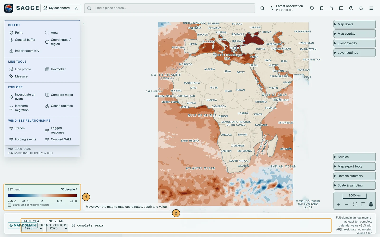
- 1Diverging legend, −0.6 to +0.6 °C per decade.
- 2Trend period: start and end year.
7-day change
The difference between the latest published day and the day seven days earlier, cell by cell. The layer exists only for the latest release and needs the exact reference day; when that day is absent from the source the layer is not built rather than being computed from a neighbour. The domain summary reports the mean change over the domain and the shares of the domain that warmed by at least 0.5 °C and cooled by at least 0.5 °C.
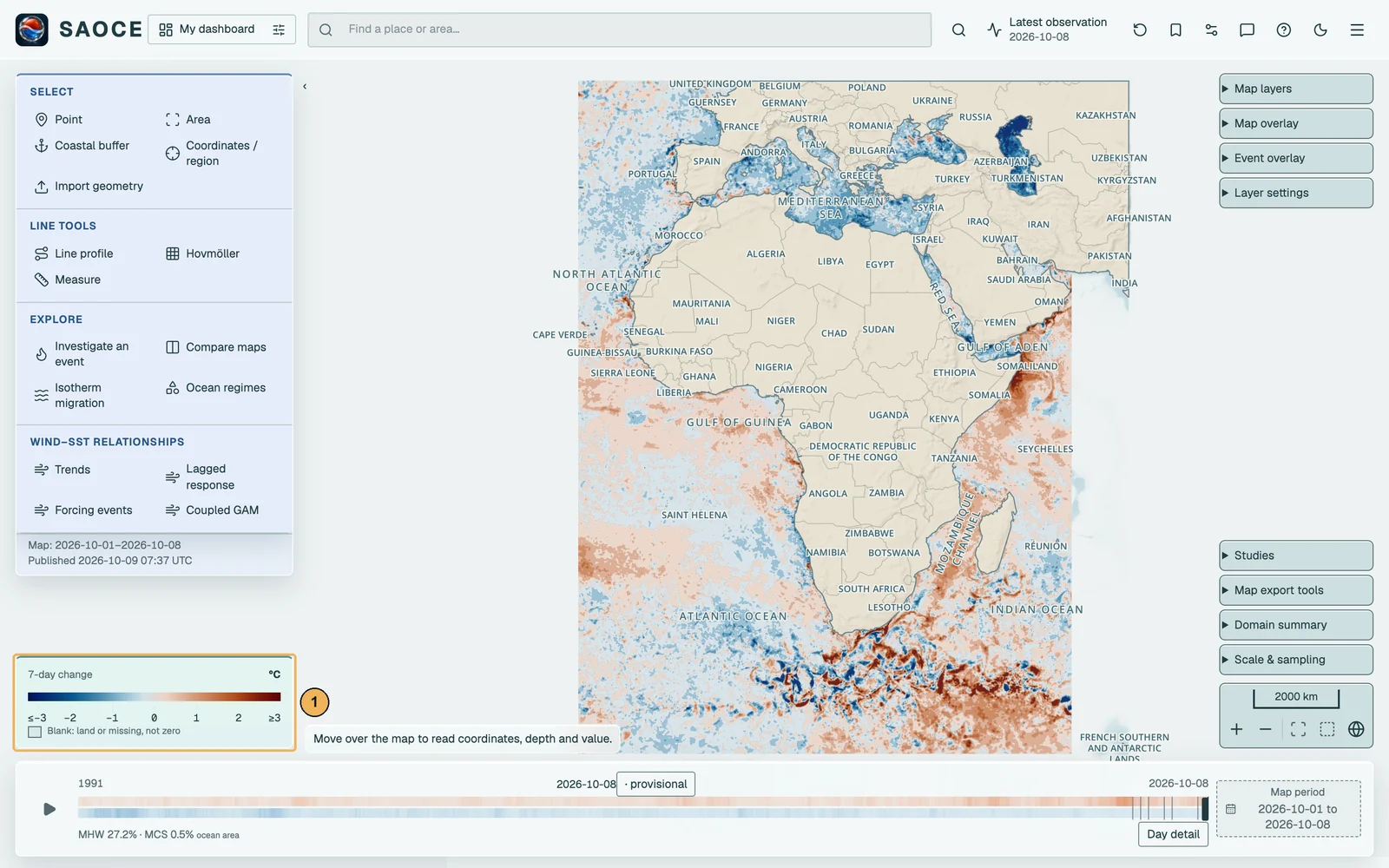
- 1Diverging legend, −3 to +3 °C.
Uncertainty
The analysis error supplied with the selected SST product, drawn on a sequential scale from 0 to 0.8 °C. It is the provider’s estimate of the standard error of the analysed SST, larger where observations were sparse or cloud-covered. The domain summary reports its median over the domain. The layer is available for the eight days of the current release.
SST gradient
The magnitude of the horizontal gradient of daily SST, by centred differences on the selected product’s native grid after a Gaussian smooth of one grid cell, in °C per kilometre with the metre-per-degree factors evaluated at each cell’s latitude. It is a display derivative that marks fronts and the edges of filaments; no front detection is claimed (decision record 0005).
Degree Heating Weeks
Accumulated heat stress after the NOAA Coral Reef Watch convention: the hotspot is daily SST minus the warmest of the twelve 1991–2020 monthly-mean climatology values of the cell, hotspots of at least 1 °C accumulate over a rolling 84-day window, and the units are °C-weeks. The layer describes the temperature product under its fixed baseline; it is not an observation of coral condition.
MHW and MCS category
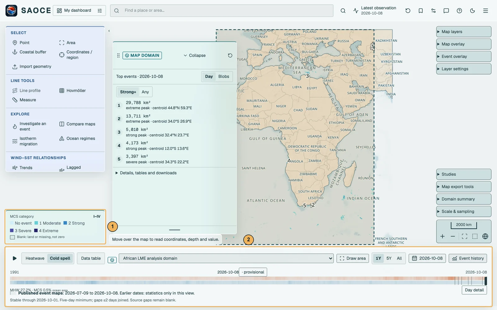
The two event layers show, for each cell, the category of the marine heatwave or cold-spell active on that day, from Moderate (I) to Extreme (IV), on the 90th-percentile and 10th-percentile definitions respectively. A cell is coloured only where a detected event is active; an isolated exceedance that does not meet the event definition is uncoloured, as is a day without source data. The detection, the categories, the event bar under the map and the spatial products are described under Marine heatwaves and cold-spells. On these layers the Top events card lists the largest contiguous patches of the day or the tracked blobs of the year.

- 1Category legend.
- 2Event bar: layer switch, reporting region, chart range, data table and date.

SST product: OSTIA or OISST
Every temperature layer, card and statistic reads one SST product at a time, chosen under Layer settings. OSTIA, the default, is the 0.05° foundation SST analysis. NOAA OISST v2.1 (AVHRR-only) is a 0.25° analysis from September 1981 held in its own archive with the same processing, its own fixed 1991–2020 climatology from heatwave3 and the same event definitions (decision record 0023). All nine SST layers, including seven-day change, uncertainty, MHWs and MCSs, use the selected product and its own availability. Event overlays and new analysis cards use that product too. Existing cards keep the product they were made with, and exports name it. The header shows the active product, native resolution and latest server date. Wind, tide gauges, ocean-regime tools and explicit OSTIA–OISST comparisons retain their separate source contracts.
OSTIA − OISST difference
Two layers compare the products on the OISST grid. OSTIA is block-averaged on request to each 0.25° OISST cell, namely the mean of the 25 native OSTIA sea cells inside it, with no interpolation, and OISST is subtracted. The daily layer shows one day; the climatology layer shows the difference of the two products’ heatwave3 1991–2020 climatologies averaged over the year or over one of the four seasons chosen under Layer settings. The domain summary gives the cosine-weighted mean, the median, the root-mean-square difference and the 5th and 95th percentiles over the shared sea cells. A difference is a product difference, not an error of either product.
difference(x, y) = mean(OSTIA cells inside the OISST cell at x, y) − OISST(x, y)