Help and methods · 9

Profiles, sections and points

The line tools read the map along a line rather than over an area. Each result opens in a floating line card beside the map, which can be dragged, expanded and closed, and which stays open while point, area and buffer cards are added. A line profile reads the displayed map for the displayed day; a Hovmöller section reads the archive along a route through time, independent of the map; the measure tool gives a distance; isotherm migration compares a monthly contour across years. Points are selections like areas and buffers, each a linked card.

Line profile

Line profile takes a start and an end point and samples the displayed grid along the straight line between them: the 0.1° display grid for Temperature and Uncertainty, and the seven-day difference for 7-day change. The line is sampled at between 24 and 180 steps, about one per 8 km, the nearest cell is taken at each step, and consecutive repeats of the same cell are dropped. The horizontal axis is the great-circle distance from the start. Land and missing cells remain gaps. The card gives the observed range, the line length and the number of valid samples; its downloads and graph options export the samples and the figure.

Hovmöller section

Click a date inside a Hovmöller to show it on the map. Scroll over the diagram to zoom around the pointer, or drag with the hand pointer to move the visible dates. Calendar plots on other cards follow the same window; Home restores all linked plots. Navigation uses the loaded cells and keeps the section’s analysis period unchanged. See timeline controls.

1. Press Hovmöller and click the start and the end of the section. Typed coordinates work in the same way. Repeat to accumulate up to four sections, labelled H1 onwards. Close a section to free a slot; its neighbours remain unchanged.
2. The route is chosen automatically and the section is built for the default settings: SST over the two years ending on the latest available day for the selected SST product.
3. Open Section settings to change the route, the buffer, the variable, the window or the end date, then press Update section. Drag the bottom handle or enlarge the card for a taller diagram; its width stays the same as other result cards.

Use Add Hovmöller above the cards to draw another section. Arrange places all open cards over the map; Dock cards puts them in the scrolling card collection. These controls also work when only Hovmöllers are open. Each section retains its own product, dates, route, buffer, variable and completed result through layout changes. The map shows a labelled route for each section. Changing the map’s SST product applies to new sections; existing cards retain the product shown in their context line.

The section reads its product’s native archive cube on the server (0.05° OSTIA or 0.25° OISST) and is independent of the displayed layer and date. Three routes exist. A straight section between the two points is snapped to a zonal line at the mean latitude when it lies within 10° of east–west, to a meridional line at the mean longitude when within 10° of north–south, and is otherwise oblique; it is sampled at up to 400 nearest cells with consecutive duplicates removed, and its axis is longitude, latitude or distance accordingly. A coastal section follows the coast between the two points, as the coastal buffer does, sampling cells within the chosen offshore buffer and labelling the axis in distance along the coast. Automatic chooses the coastal route when both endpoints lie within 25 km of the same coastline and are at least 10 km apart, and the straight route otherwise.

The variable is SST, on the fixed 10 to 29 °C scale, or the SST anomaly against the 1991–2020 heatwave3 day-of-year climatology, on the ±5 °C scale. The window is one, two, five or ten years ending on the chosen end date, which must keep the whole window inside the archive. Time runs along the horizontal axis with year ticks; the vertical axis is the route position, both titled with their units. The time axis is a regular daily calendar, so a source-absent day is a blank column, and no value is interpolated in either direction. A request beyond 1.5 million samples is refused with a message to shorten the window or the section.

Measure

Measure takes two points and reports the great-circle distance between them on a sphere of mean radius 6,371.0088 km, to two decimals below 10 km and to one decimal otherwise, together with the two coordinates.

Isotherm migration

Isotherm migration, under Spatial change in the left workspace, draws the contour of a chosen monthly-mean temperature (15, 18, 20, 23 or 26 °C, 20 °C by default) for a chosen month in each year, so that a poleward or equatorward displacement over the years can be seen on the map. A month enters only with at least 90% of its days observed, and nothing is interpolated. It is a visual counterpart of warming, not a fitted trend.

Histogram

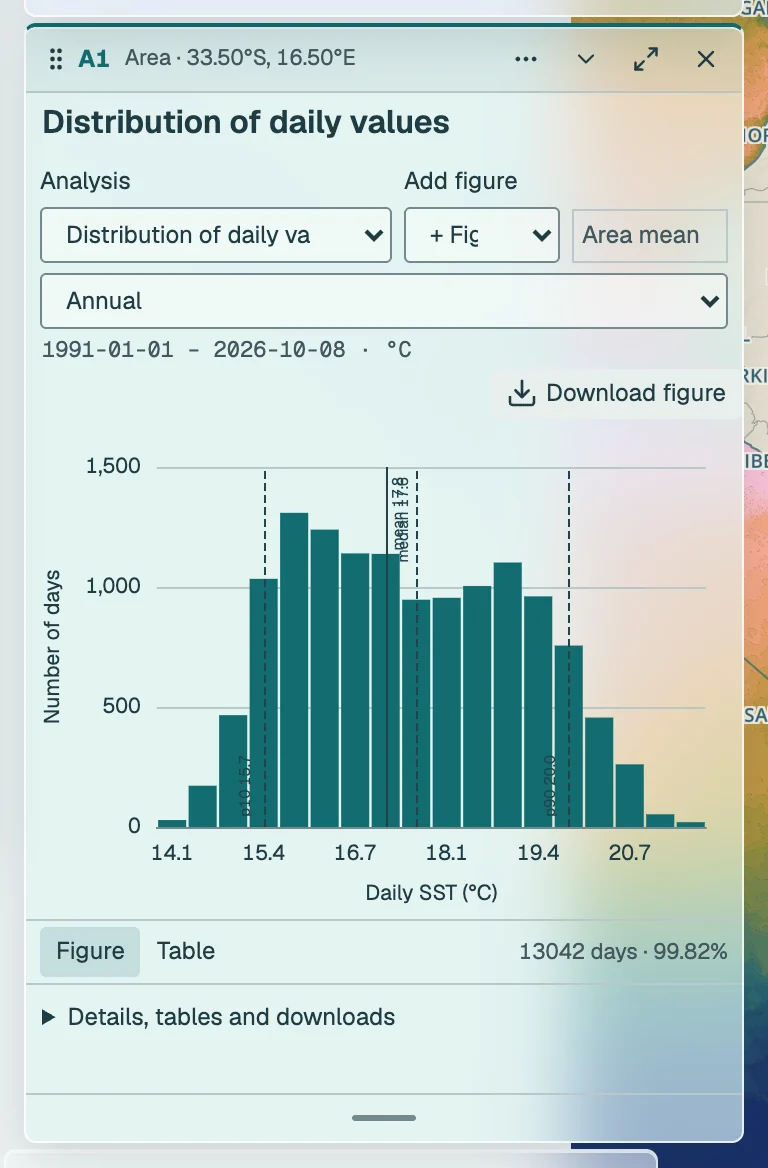
Distribution of daily values is a method on every card, under What are the conditions?. It bins the selection’s daily values over the analysis interval into equal widths between the observed minimum and maximum, with the bin count the square root of the day count held between 8 and 18, and marks the mean and median. For an area or buffer each day is already the cell-area-weighted mean, so the histogram describes time, not space. Missing days are left out, never filled.

Linked point analyses

Every point click after Point adds a compact point card. Choose 1, 4 or 16 native native pixels (0.05° OSTIA or 0.25° OISST), displayed as a fixed 1×1, 2×2 or 4×4 footprint. Temperatures use a spherical-cell-area-weighted mean with at least 90% of the fixed ocean area present. Land and missing cells are never replaced by a different ocean location.

Choose a question and a method on the card. Linked cards share the method and its scientific settings unless independent analyses are enabled.

The shared interval applies to the linked point, area and buffer cards; incomplete calendar years are excluded from annual fits. Expand a card for its main figure, selectable additional figures, method settings and display layers. Detailed statistics, data and provenance are collapsed below. Chart comparison & downloads includes the paired trend-difference test for two selected cards. Arrange, Minimise all and Dock cards include the open line-tool card and keep the map accessible while markers stay linked. Hovmöller and other line tools retain their own dates and settings.

For multiple pixels, the uncertainty line is a conservative upper bound formed from weighted source standard errors under perfect positive correlation. It is not an independence-based standard error or confidence interval. Unarchived uncertainty stays unavailable. Save analysis reconstructs the full point group, its exact footprints, fixed interval and per-card settings.